Chapter 3: Design Of Experiments
- Rakshan Bathri
- Feb 1, 2025
- 18 min read
Updated: Feb 2, 2025
Chapter 3.1: Introduction to DOE!
Doe re mi fa so la ti doe
Welcome Back👋👋 As I'm writing this, it's Chinese New Year 🧧, so…Gong Xi Fa Cai❗ Hope everyone reading this had a great time visiting relatives, collecting ang baos 💰, and enjoying all the good food 🍍 instead of being stuck with things like a blog, CEDCS Assignment 2, SIP, or that dreaded EWW report draft 😩. (this cny not really new year-ing)
Q: "What is DOE❓"
A: DOE stands for Design Of Experiments 🔬❗ We engineers will definitely be doing TONS of experiments 📊. One dreaded experiment that we’ll all have to face is our Final Year Project (FYP) 😨. Now, you might be wondering why I’m bringing up FYP...that’s because it’s OUR FYP, meaning there’s no practical manual 📖 to follow. We’ll have to design the experiments ourselves 🛠️.
Since I have no clue what we’ll be doing for our FYP, let’s use the microwaving of popcorn 🍿 as our main experiment. This also happens to be the case study I was given.
For those who have made popcorn before, I’m sure you’ve noticed there are always a few unpopped kernels😭 Did you know these unpopped kernels are actually called bullets 💥❓
(I didn’t even know that, ngl 😅). We all hate having bullets in our popcorn, right❓ So, how can we reduce the number of bullets❓ By adjusting the microwaving process❗❗
Basically, DOE allows us to design an experiment involving multiple factors to obtain the best possible and optimised process 🔬❗ You might also be wondering why we can’t just increase the microwaving time or something similar ❓ Well, that’s because not only will your popcorn get burnt 🍿🔥, but there may also be interaction effects between other factors (I’ll talk more about this later)❗
Not only that, but without keeping track of what you’re experimenting with, it won’t really be optimised, will it❓ Why❓ Because you’re probably going to forget what you changed, or you might even repeat the same experiment twice 🔄❗
Hence, DOE is a statistics-based approach 📊 to designing experiments, allowing us to systematically investigate the effects of multiple factors on a given process ❗ It provides a structured way to obtain valuable insights into complex, multi-variable processes while using the fewest trials possible 🔍. (this is from the slides btw LOL)
Rather than relying on trial and error, DOE helps engineers optimise the experimental process itself, ensuring that every experiment conducted contributes meaningfully to understanding the system ❗ This makes DOE an essential tool in not just product design 🏭 but also in process improvement, where efficiency, consistency, and quality control are critical 🔧.
By applying DOE, engineers can fine-tune processes, identify key influencing factors, and eliminate unnecessary variables, ultimately leading to better performance, cost savings, and innovation 🚀. Whether it’s reducing defects in manufacturing, enhancing chemical reactions, or even perfecting the art of making popcorn, DOE provides a data-driven approach to achieving the best possible outcome❗
You now have a basic understanding of DOE 🎉❗ Now, let’s dive into our case study on microwaving popcorn 🍿 to see how we can use DOE to optimise the process❗
There will be three key factors that we’ll be focusing on:
🔹 Diameter of bowls (Factor A)
🔹 Microwaving time (Factor B)
🔹 Power setting of the microwave (Factor C)
Since our goal is optimisation, we can’t just randomly experiment. We need to systematically vary the factors to understand their effects❗ To do this, we will assign two levels for each factor:
High (+) – A higher value of the factor
Low (-) – A lower value of the factor
Fortunately🙏 in the case study, we were given the High and Low values of each factor❗
Factor | Low (-) | High (+) |
Diameter (A) | 10cm | 15cm |
Microwaving Time (B) | 4 minutes | 6 minutes |
Power (C) | 75% | 100% |

By carefully selecting and controlling these levels, we can identify the best combination that minimises the number of unpopped kernels (bullets 💥) while ensuring the popcorn is perfectly cooked! 🍿 To achieve this, we need to gather the data from every possible combination of these factors. Since this has already been provided and I've plotted it in Excel, here’s a screenshot with the information you need! 📊👀
(FYI, 8 runs were performed with 100 grams of corn used in every experiment and the measured variable is the amount of “bullets” formed in grams)
(that was one long introduction)
Chapter 3.2.1: Full Factorial Design!
time to analyse
Full Factorial Design❓
Full Factorial Design is a powerful approach used in the DOE, where we gather data from every possible combination of the factors we’re investigating. When I mentioned, "we need to gather the data from every possible combination of these factors" I was referring to this exact method❗ This design is ideal when we want to thoroughly explore all potential outcomes and truly discover the best combination for optimising a process. In this case, something like microwaving popcorn 🍿✨
The advantage of using a Full Factorial Design is that it allows us to study the main effects (individual impacts of each factor) and the interaction effects (how factors work together)❗ By testing every combination, we can be sure that we’re not missing any crucial relationships between variables that could affect the outcome. The more data we gather, the more accurate our results are, and we gain a deeper understanding of how each factor contributes to the final result 📊💡
This design becomes especially useful in processes with multiple factors, where interactions between those factors might have a significant impact❗ Without a Full Factorial Design, we'd only look at individual factors in isolation, potentially missing out on important insights❓🔍
However, you might be wondering, why don’t we just use the Full Factorial method for everything❓ Well, the reason is that it can be too time-consuming and resource-intensive 💼. Running experiments for every possible combination of factors means you’ll need lots of time, resources, and sometimes even extra help to gather and process the data. ⏳⚙️ On top of that, it can lead to a data overload, making it tricky to sift through and interpret all the information effectively 😵.
So while the Full Factorial method is super thorough, it might not always be the most practical choice, especially if we’re dealing with a large number of factors or limited resources!
Thankfully, we only have 8 runs, and the data is already given above 📊✨. So now, it's time to analyse and uncover some insights❗ Let's dive in and make sense of the data to find the best combination for those perfectly popped kernels! 🍿🔍
Chapter 3.2.2: Individual Factors!
the single effects and its ranking


Here is all the data that we will need for reference 📊.
Q: "What can we conclude from the data above❓"
A: We can determine the effect of single factors❗ 💡 By looking at how each factor influences the outcome, we can identify which ones have the most significant impact on achieving the perfect popcorn❗ 🍿
Analysis:
Diameter of Bowl (Factor A)
When we increase the diameter of the bowl from 10 cm (Low Level) to 15 cm (High Level), the mass of bullets decreases from an average of 1.70g to 1.55g❗🎉 This means that 0.15g more kernels (I don't know why but this sounds weird) were popped, which translates to more popcorn! 🍿✨ A clear win❗ Looks like a bigger bowl is the way to go❗
Microwaving Time (Factor B)
Likewise, when we increase the microwaving time from 4 minutes (Low Level) to 6 minutes (High Level), the mass of bullets also decreases from 2.07g to 1.18g❗🍿 This means we got an additional 0.89g worth of popcorn❗🎉 Hence, this clearly shows that a longer microwaving time is better for getting more popcorn✅
Power Setting of the Microwave (Factor C)
When we increase the power from 75% (Low Level) to 100% (High Level), the mass of bullets decreases from 2.63g to 0.62g✨⚡ This results in the most significant change among all the factors, providing us with an extra 2.01g worth of popcorn! 🍿🎉 So, cranking up the power really makes a big difference in getting those kernels popped! 💥 (this sounds so cliche)
However, it isn't a true analysis without a graph📈 Why❓ Because we need to determine trends as well❗ Visualising the data helps us spot patterns and better understand the relationships between the factors and the amount of popcorn we get. It makes the analysis clearer and more insightful! ✨ Let's plot those trends and get a full picture of how each factor is influencing the results❗ 🍿


Final ranking of the significance of each factor:
Power Setting > Microwaving Time > Diameter of Bowls
⚡>⏱️>🍽️
From the graph, we can easily visualise the overall trend of what changing each factor does! That is, when we change a factor's level from low to high, in general, the mass of bullets decreases! 📉🍿
Even though we’re given the data to determine the significance of each factor, let's just pretend we don’t have it and have to strictly infer from the graph. How would we do that❓ That's right! By analysing the absolute gradient of each graph! (So smart! 😎)
Why the absolute gradient? Because it tells us how much changing a factor can affect the mass of bullets left. For example, for a significant factor like power, with even a small increase, we can infer that the mass of bullets will drop much more drastically compared to a similar increase in a factor like the diameter of bowls! 📊⚡
So how do we see the gradient❓ As engineers, we should all know the equation Y = mX + C, where m is the gradient! In the graph, we can observe the gradient of each of the lines according to their colour. 🎨
Diameter – Blue (absolute gradient = |-0.15|)
Microwaving Time – Orange (absolute gradient = |-0.89|)
Power – Grey (absolute gradient = |-2.01|) (grey would blend in with the background so I just put black)
This shows that the power setting of the microwave is indeed the most significant factor, followed by microwaving time, and lastly the diameter of the bowls❗
But before I proceed with the next section, do you wonder why we need to look at the absolute gradient and not just the normal gradient❓🤔 Well, that’s because, in other experiments, not all factors have the same trend as ours❗❗ For example, let’s say Factor A has a gradient of 2 and Factor B has a gradient of -10. If we don't take the absolute gradient, we might wrongly conclude that A > B and that A is more significant, which is totally misleading! ❌
Hence, we need to take the absolute gradient instead, so we can correctly compare the magnitude of change for each factor, regardless of whether it’s a positive or negative trend! ✅
Chapter 3.2.3: Interaction Effects
How does A & B & C affect each other?
(I just want to say that unlike the rest I actually listened during class 🤯🤯 #benefitsofseatingfrontrow)
The next thing we need to do is find the interaction effects between each factor. 🔄
Let’s start with the interaction effect between Diameter (Factor A) and Microwaving Time (Factor B), or A x B.
First, we need to pull up our data table again 📊 so we can examine the relationship between these two factors and how they interact with each other. Ready? Let’s dive in! 😎 (cliche.)
Since we are finding the interaction between A (Diameter) and B (Microwaving Time), we need to set A as the base. This means we need to find the average mass of bullets left when A is at both low and high levels, for both low and high levels of B.
I know it sounds a bit confusing, so here’s the table to make it easier to visualise 📊. This will help us see how the interaction between the two factors affects the results! 👀

Next, we need to plot a graph like the one below❗

Two factors are said to interact when the effect of one factor on the response variable changes depending on the level of the other factor. 🔄
As you can see from the graph above 📊, the gradients of both lines are different. One is + and the other is -. This shows that the effect of Diameter of the Bowl (A) and Microwaving Time (B) on the mass of bullets varies at different levels. 📉📈 (You can spot the gradient of each graph on the right side of the image above.)
This difference in gradients confirms a significant interaction between A (Diameter of the Bowl) and B (Microwaving Time)❗💥
Next, we will look at the interaction effect between the Diameter of the Bowls (Factor A) and Power (Factor C), or A x C❗
We'll follow a similar approach as before to determine how these two factors interact and influence the mass of bullets. So I won't be explaining too much in detail.


As you can see from the graph above 📊, the gradients of both lines are different. One is + and the other is -. This shows that the effect of Diameter of the Bowl (A) and Power Setting (C) on the mass of bullets varies at different levels. 📉📈
This difference in gradients confirms a significant interaction between A (Diameter of the Bowl) and C (Power Setting)❗💥
Next, we will look at the interaction effect between the Microwaving Time (Factor B) and Power (Factor C),
or B x C❗


As you can see from the graph, the gradients of both lines are different, but by only a small margin. 📊 This indicates that there is an interaction between Microwaving Time (Factor B) and Power Setting (Factor C), but the interaction is relatively small.
Chapter 3.2.4: Conclusion
what can we infer?
From our analysis, we can conclude that Power Setting is the most significant factor, followed by Microwaving Time, and then Diameter of the Bowl ⚡🍿. To achieve the highest yield of popcorn, all factors should ideally be set to their high levels. 🎯
However, we must consider the significant interactions between factors. The gradients for A x B (Diameter of the Bowl and Microwaving Time) and A x C (Diameter of the Bowl and Power Setting) show that at high levels, the interaction effect is stronger, meaning changes in one factor can lead to bigger changes in the outcome. 📉📈
Therefore, while high settings may seem ideal, we need to find an optimised value that accounts for these interactions. By testing different combinations, we can determine the balance that gives the best popcorn yield without overemphasising any one factor. 🔄💡
Chapter 3.3.1: Fractional Factorial Design!
round 2!!! yipee
Fractional Factorial?
Remember the cons I mentioned earlier about using a Full Factorial Design❓ One of the main issues is the time and resources required to complete all the runs. This is where Fractional Factorial Design comes in❗❗ As the name implies, we only use a fraction of the dataset, meaning we don’t need to conduct all 8 runs to get meaningful results! 🎯
By choosing fewer than all possible treatments, we can still gather sufficient information to determine the factor effects, making the process more efficient and resource-effective. 📊 However, the trade-off is that there’s a risk of missing some information, so while it’s quicker, we need to be careful not to overlook important details. ⚖️
For our fractional factorial design, we only need 4 runs, which helps us balance efficiency with accuracy! 💡
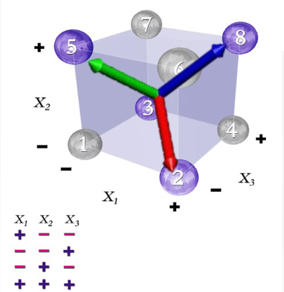
Q: "Which runs do we pick❓"
A: Let's imagine a (x, y, z) plot in the shape of a cube like the one on the left. (I’m having PTSD from advanced math right now 😅). To "get the best of all 3 worlds" (where "worlds" are the factors), we would need to assume an orthogonal shape.
Orthogonal basically means that each point is perpendicular to another. By doing this, we ensure that all factors (both low and high levels) occur the same number of times, which gives us a balanced and efficient design. Plus, it has good statistical properties, meaning we can get reliable results without overcomplicating things! 📊✨
Hence, the runs we will pick will be Run No. 1, 2, 3, and 6, as they match the high and low values shown in the picture. The Statistical Orthogonality method can be used here because it is a balanced design that ensures all three factors, Diameter, Microwaving Time, and Power, occur the same number of times. This way, each factor is varied at least once, and we can draw a fair conclusion from the results! 📊💡
Hence, here is our new data table! 📊✨

This table reflects the 4 runs we selected using the Statistical Orthogonality method, ensuring that all three factors are covered and balanced for analysis. Let's dive in and explore the results! 🚀 (it's so cliche that I just find it funny atp)
Chapter 3.3.2: Individual Factors!
the single effects and its ranking. again.

(I forgot to divide by 2 instead of 4 in my first draft LOL)
As mentioned earlier for the Full Factorial Design, we can determine the effect of single factors❗💡 By examining how each factor influences the outcome, we can identify which ones have the most significant impact on achieving the perfect popcorn❗🍿 This allows us to pinpoint the key factors that truly make a difference in popping that perfect batch! 🎯
Analysis:
Diameter of Bowl (Factor A)
When we increase the diameter of the bowl from 10 cm (Low Level) to 15 cm (High Level), the mass of bullets INCREASES from an average of 1.61g to 1.90g❗ This means that 0.29g fewer kernels were popped, which translates to less popcorn. 😕 This isn't ideal for us, as we want to maximise the popped kernels and get the most out of our popcorn❗🍿
Microwaving Time (Factor B)
When we increase the microwaving time from 4 minutes (Low Level) to 6 minutes (High Level), the mass of bullets decreases from 2.11g to 1.40g✨. This means we get an additional 0.71g worth of popcorn! 🎉 This clearly shows that longer microwaving time leads to more popcorn! ✅
Power Setting of the Microwave (Factor C)
When we increase the power from 75% (Low Level) to 100% (High Level), the mass of bullets drops from 2.97g to 0.53g! ⚡ This leads to the largest change among all the factors, giving us an extra 2.44g of popcorn! 🍿🎉 Clearly, increasing the power has the biggest impact on getting more kernels popped! 💥(this sounds so cliche)
Just like before, we’re plotting a graph again to help us visualise the data! 📊 Why is this important❓ Because it lets us clearly see the trends and relationships between the factors and the amount of popcorn we get. By visualising the data, we can spot patterns that might be hard to see in just numbers alone, making the analysis more insightful and easier to understand! ✨ Let's plot these trends and get a clearer picture of how each factor is influencing the popcorn yield! 🍿

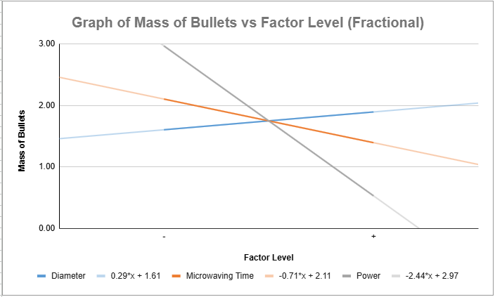
Final ranking of the significance of each factor:
Power Setting > Microwaving Time > Diameter of Bowls
⚡>⏱️>🍽️
From the graph, we can see that as both microwaving time and the power setting increase, the mass of bullets decreases. This makes sense, as more time and power lead to better popping of the kernels! However, when the diameter of the bowl increases, the mass of bullets actually increases, meaning fewer kernels are popped. This is a bit counterintuitive but shows that a larger bowl might not be the best choice for maximising popcorn yield! 🍿
Diameter – Blue (absolute gradient = |0.29|)
Microwaving Time – Orange (absolute gradient = |-0.71|)
Power – Grey (absolute gradient = |-2.44|)
This shows that the power setting of the microwave is indeed the most significant factor, followed by microwaving time, and lastly, the diameter of the bowls❗ Why❓ Because of the absolute gradients! (I'm not going to waste your time by telling you the whole explanation again so you can click here to go back) But let me add to my explanation here. If we didn't take the absolute gradients, it would incorrectly suggest that the diameter of the bowls is the most significant factor, which is false! ❌ That’s why using the absolute gradient is crucial to get an accurate understanding of the impact of each factor! ⚖️
Q: "Is there any reason for the difference in trends❓
A: Yes❗ Remember the one con I mentioned about using the Fractional Factorial method❓😅 We risk losing some information 🧠, and it’s generally less reliable than the full factorial approach. This is likely why we saw a different result for the diameter of the bowls. The reduced number of runs in the fractional design might have missed some key interactions, leading to this unexpected trend❗🤔
Chapter 3.3.3: Interaction Effects
How does A & B & C affect each other? again.
Time for the interaction effects again! Since we’re already familiar with the process of getting the values, I’ll skip straight to showing you the table and graph 📊


The gradients of both lines are different (one is + and the other is -), and there’s an intersection between them. 📉📈 This indicates that there’s a significant interaction between Factor A (Diameter of the Bowl) and Factor B (Microwaving Time)❗ (A x B)


As you can see from the graph above 📊, the gradients of both lines are different. One is + and the other is -, meaning the effect of Diameter of the Bowl (A) and Power Setting (C) on the mass of bullets varies at different levels. 📉📈 This difference in gradients confirms a significant interaction between A (Diameter of the Bowl) and C (Power Setting)❗ (A x C)


As you can see from the graph 📊, the gradients of both lines are different, but only by a small margin. This indicates that there is an interaction between Microwaving Time (Factor B) and Power Setting (Factor C), but the interaction is relatively small compared to the others. 🔍 While they do influence each other, the effect isn’t as strong as the previous interactions! (B x C)
Chapter 3.3.4: Conclusion
how do the results vary?
From our Fractional Factorial Design, we can still determine that the power setting is the most significant factor, followed by microwaving time, and lastly, the diameter of the bowl❗ The best settings for achieving the highest popcorn yield, according to this method, would be:
Power: 100% (High Level) ⚡
Microwaving Time: 6 minutes (High Level) ⏳
Diameter of Bowl: 10 cm (Low Level) 🍲
This is different from what we concluded in the Full Factorial Design, where increasing the diameter of the bowl led to fewer unpopped kernels. This difference is likely due to the loss of information when using the Fractional Factorial Design, making it less reliable compared to the Full Factorial Design. 😵💫 Since we only tested half the total runs, certain interactions may have been missed or misrepresented.
While Fractional Factorial Design is faster and more resource-efficient 🏎️, it comes with trade-offs in accuracy. To get the best possible settings, we would ideally balance efficiency with reliability by testing additional runs to confirm the trends we observed❗📊
Chapter 3.4: Reflection Time
final stretch
Not gonna lie, this blog was the hardest for me to write about, not because of its difficulty but because I'M REALLY NOT SURE WHAT TO INCLUDE. There wasn't much info given about DOE itself so I had to do my own research but at the same time, I didn't want to waste too much time since its only 5%. So, I did what anyone else would do and just wrote about what I knew. #kiasu.
Okay, reflection time.
Initial Thoughts on DOE
At the start of the tutorial lessons on Design of Experiments (DOE), I struggled to understand why we needed to learn about it in the first place. It seemed intuitive, something we already applied in everyday life without formal training. For example, when making cup noodles, if we find them overcooked, our instinct is to reduce the microwave time. However, through the Lactose Dissolution case study, I realised that DOE is essential for complex processes where multiple factors influence the outcome. In such cases, a simple trial-and-error approach is not sufficient. While DOE can still be applied to something as straightforward as cooking noodles, it may not always be necessary when a quick Google search can provide the answer.
Understanding the Trade-offs Between Full and Fractional Factorial Designs
The discussion on Full vs. Fractional Factorial Designs highlighted the importance of choosing the right approach depending on the context and constraints. A full factorial design provides the most accurate and comprehensive insights, which makes it ideal for situations where precision is critical. This would apply to fields like pharmaceuticals or chemical extractions, where errors could lead to significant consequences. However, in cases where speed and efficiency matter more, such as optimising a recipe, using a fractional factorial design makes more sense. By reducing the number of experiments, we can still obtain valuable insights while saving time and resources. This reinforced an important concept: accuracy, time, and resources are always in balance. The choice of DOE method depends on what trade-offs we are willing to make.
Applying DOE in Practical Sessions
The catapult experiment was a great example of how DOE can be applied to real-world problem-solving. We had to analyse data and adjust factors such as catapult arm length to optimise our shots. My group finished in second place. Looking back, we could have won if we had not attempted to hit two targets at once, a strategic mistake that cost us precision. This experience reinforced the value of using DOE to make data-driven decisions rather than relying purely on intuition.
Recognising Higher-Order Interactions and the Importance of Graphs
One of the biggest takeaways from the practical session was my realisation that higher-order interactions (such as second-and third-order effects) were not covered in detail, yet they appeared in the Excel sheet. This made me aware of the depth and complexity of DOE that I had not fully considered.
More importantly, I learned that graphs play a crucial role in visualising interactions. Without them, I would not have realised how different factors interact. For instance, in our microwave popcorn case study, while it may seem logical that increasing both power and microwaving time would always result in more popcorn, the reality is more nuanced. Excessive heat could burn kernels instead of popping them, demonstrating an unexpected interaction between the factors. Seeing the interaction effects clearly on a graph helped me understand that analysing trends visually is just as important as looking at numerical values when interpreting experimental results.
Applying DOE to My Internship and Final Year Project
DOE will be particularly useful in my upcoming internship, where I will be conducting small-scale experiments before they are upscaled for larger production. In an industrial setting, testing every possible combination is impractical due to time and cost constraints. Because of this, I expect to use fractional factorial designs to identify the key influencing factors. Understanding interactions between variables will be crucial to ensuring that the process works efficiently when scaled up.
Similarly, for my Final Year Project (FYP), DOE will help in structuring my experiments effectively. Instead of changing one factor at a time, I will be able to systematically test multiple factors and determine their combined effects. This approach ensures that I reach the optimal conditions with fewer trials. Visualising the results using graphs will also be essential, as they will allow me to quickly identify trends and interactions that might not be obvious from raw data alone. The lessons from this module have shown me that designing experiments strategically is just as important as the experiments themselves, and I intend to apply these learnings to future projects.
Here are the files :)
apologies for the lengthy blog ms tan😭
BYEBYE TY FOR READING❗✨😵


Comments